Research Note
Pricing Before Prediction: How to Build and Test a Credit Engine
Preview prompt
Summarize the Ionitsa research note titled "Pricing Before Prediction: How to Build and Test a Credit Engine" for a technical reader.
Cover the problem or research question, implementation or method, evidence or results, and limitations.
Separate facts stated on the page from your own assessment, note anything unclear or unverified, and avoid promotional language.

Primary source: https://ionitsa.com/research/pricing-before-prediction-credit-guide.md
Canonical page: https://ionitsa.com/research/pricing-before-prediction-credit-guide/
A practical guide to bootstrapping CDS hazard rates, pricing fixed-rate bonds, validating the numerical machinery, and knowing when linear credit P&L has stopped being reliable.
Credit research often begins one layer too late.
A spread looks cheap against its history. A bond appears wide to CDS. A cross-sectional model ranks one issuer above another. The notebook moves quickly to signals, Sharpe ratios and charts—while price, survival probability, recovery and hedge sensitivity remain fields supplied by somebody else’s system.
That is enough to explore an idea. It is not enough to demonstrate that the instrument itself is understood.
This guide builds the missing layer: a small CDS hazard-curve engine and a fixed-rate bond Z-spread engine, surrounded by tests. It then uses full revaluation to measure when the familiar linear P&L approximation begins to mislead a bond–CDS hedge.
The objective is not to recreate a bank’s production library in a notebook. It is to make every economic sign, numerical solver and model limitation visible before the output is allowed into a strategy.
Model disclosure: The Python implementation is an independent educational model informed by standard CDS economics. It is not the ISDA CDS Standard Model and is not represented as ISDA-conformant. Contractual valuation should use the official model, documentation and test grids.
Data disclosure: The calibration quotes and spread shocks below are deterministic scenarios, not historical market observations. They test the engine and expose approximation error; they do not establish expected return.
The stack we are going to build
The calculation has four layers. Their order matters.
flowchart LR
  A[Discount factors] --> B[Hazard curve]
  B --> C[CDS cash-flow valuation]
  A --> D[Bond cash-flow valuation]
  C --> E[RPV01 and full CDS P&L]
  D --> F[Z-spread, DV01 and CS01]
  E --> G[Model-consistent hedge]
  F --> G
  G --> H[Strategy research]
The discount curve values certain cash flows. The hazard curve turns CDS quotes into risk-neutral survival probabilities. Those two curves value the CDS premium and protection legs. The bond engine discounts contractual cash flows with an additional spread. Only then can a researcher compare full-revaluation P&L with the first-order sensitivities used for hedge sizing.
Step 1: represent the discount curve explicitly
Let be the continuously compounded zero rate to maturity . The discount factor is:
The teaching implementation linearly interpolates zero rates between declared nodes and holds the end rates flat outside the node range. That is deliberately plain. The important design choice is that discounting is its own object with tests: , time cannot be negative, and a positive flat curve produces decreasing discount factors.
A production implementation would construct the applicable OIS/RFR curve from market instruments using the currency-specific conventions in the official ISDA curve specification. It would not silently substitute a five-year Treasury yield for an entire discount term structure.
Step 2: convert CDS spreads into a survival curve
Assume default time has a piecewise-constant risk-neutral intensity . Survival to is:
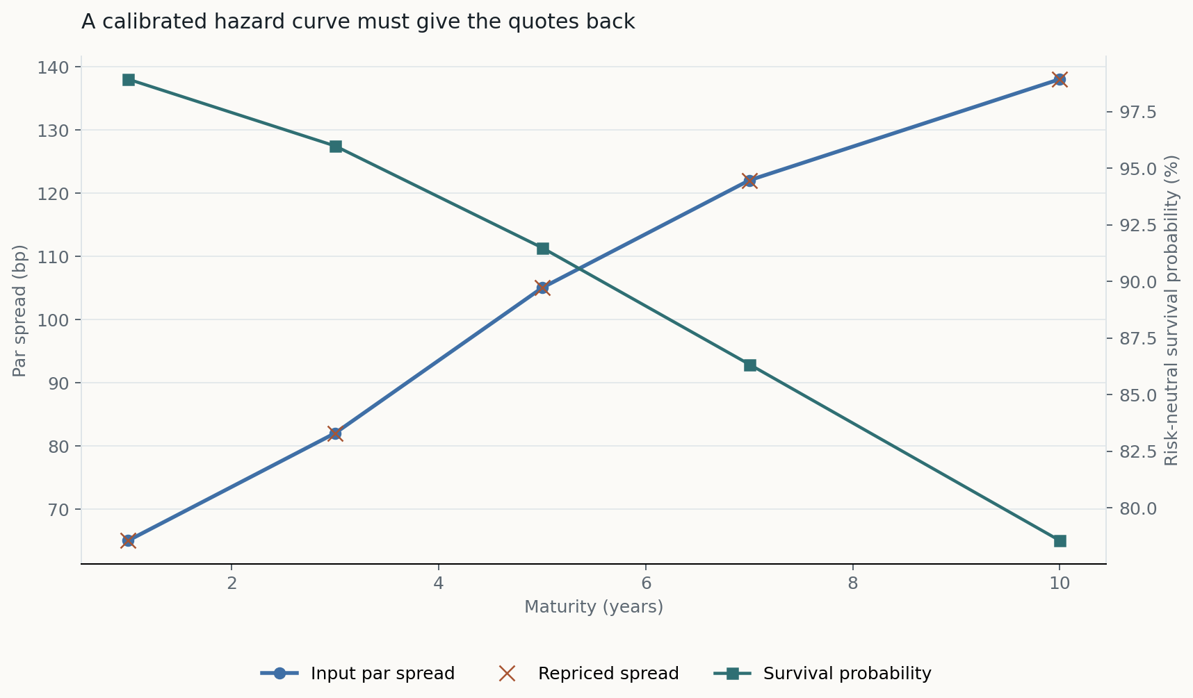
With nodes at one, three, five, seven and ten years, the engine solves one hazard rate for each interval. The one-year quote determines the first hazard. Holding that result fixed, the three-year quote determines the second, and so on. A bracketed bisection solver is slower than a clever method and much easier to audit.
The essential calibration test is not that the hazards look plausible. It is that the curve gives every input quote back.
The maximum absolute repricing error in this run is below basis points. That tolerance does not make the model institutionally complete. It only shows that the numerical bootstrap solves the model it was given.
Step 3: price the premium and protection legs
A protection buyer pays the contractual coupon while the reference entity survives and receives loss given default if a covered credit event occurs. Ignoring contractual date detail for the moment, the protection leg is:
where is notional and is recovery.
The risky premium annuity contains scheduled coupons plus premium accrued between the previous coupon date and default:
For coupon , the protection buyer’s value is:
The par spread sets that value to zero:
Risky PV01 follows immediately. It is the value of one basis point of contractual premium:
This identity gives three high-value tests. A CDS struck at its par spread must have zero value. RPV01 must agree with a one-basis-point coupon finite difference. At low hazards and flat conditions, the result must approach the familiar approximation .
Standard North American and European CDS trade with fixed coupons and an upfront amount. The guide engine converts between the two by valuing the fixed-coupon contract on the calibrated curve. The official converter exists because counterparties need those upfront calculations to match; its specification also makes clear how much date, accrual and calendar machinery the simplified equations omit.
Step 4: price the bond independently
For a fixed-rate bullet bond with cash flows , the model dirty price at Z-spread is:
The Z-spread is the value of that reproduces the observed dirty price. The clean price is dirty price less accrued coupon. The engine checks both directions: price from a known spread, then solve the spread back from that price.
Credit-spread DV01 is calculated with a central difference:
Rates DV01 bumps the underlying zero curve instead. Keeping those sensitivities separate prevents a bond’s rates exposure from being mistaken for credit hedge notional.
This engine intentionally stops at fixed-rate bullets. A callable bond’s Z-spread is not its OAS. Option-adjusted valuation needs an interest-rate model, volatility assumptions and an exercise policy. Renaming the simple output would add apparent sophistication and remove accuracy.
Step 5: validate identities before comparing strategies
A pricing library should have a hierarchy of evidence.
First come internal identities:
- discount factor at time zero is one;
- survival stays inside and never rises;
- default probabilities are non-negative;
- each CDS quote reprices inside tolerance;
- par CDS value is zero;
- clean plus accrued equals dirty;
- yield and Z-spread inversion recover their inputs;
- analytic or reported sensitivities match finite differences.
Second come economic directions:
- wider CDS quotes reduce survival;
- wider bond Z-spread reduces price;
- protection struck below the market spread has positive value to the buyer;
- higher recovery reduces the protection payment for a fixed hazard curve.
Third come external golden cases. The next production gate is comparison with the official ISDA test grids and an independent implementation such as QuantLib. Dates, calendars, recovery, curve inputs, coupon and settlement convention must be identical before a difference is called a model error.
The repository currently contains 22 tests across curves, CDS valuation, bond valuation and the experiment. They are a floor, not a certification.
The experiment: when does linear P&L break?
The existing bond–CDS research used first-order spread sensitivities. That is appropriate for an auditable baseline, but the approximation should have a measured operating range.
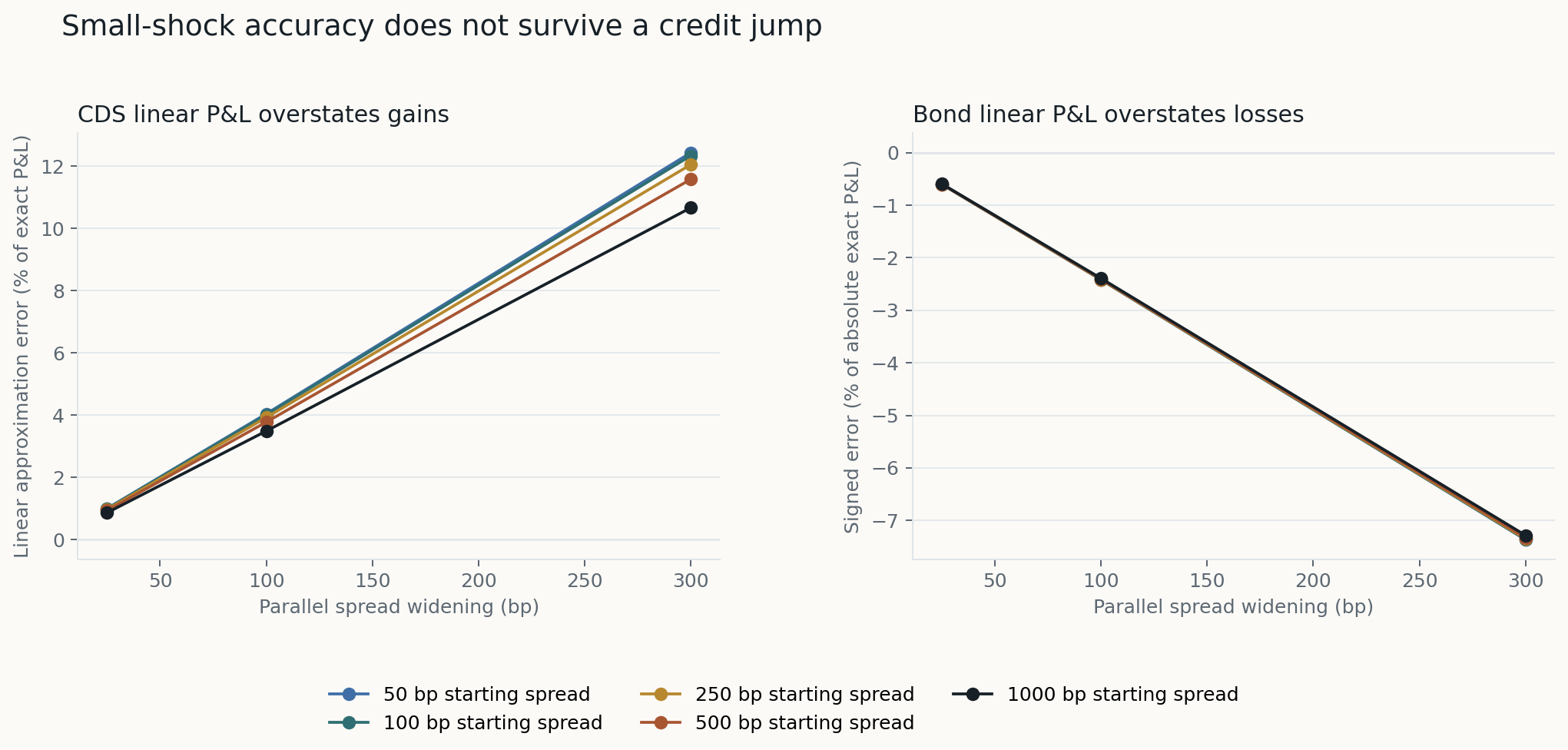
The experiment starts a five-year CDS and a five-year 5% coupon bond at spreads of 50, 100, 250, 500 and 1,000 basis points. Notional and bond face value are $1 million. Recovery is 40%. Each scenario widens the entire CDS quote curve and the bond Z-spread by 25, 100 or 300 basis points.
For the CDS, linear P&L is initial RPV01 multiplied by the spread shock. Exact P&L recalibrates the hazard curve and revalues the original coupon. For the bond, linear P&L is initial CS01 multiplied by the shock; exact P&L discounts every cash flow at the shocked spread.
| Spread widening | Maximum CDS linear error | Bond linear error |
|---|---|---|
| +25 bp | 1.00% | -0.60% |
| +100 bp | 4.04% | -2.42% |
| +300 bp | 12.43% | -7.37% |
The CDS error varies with the starting spread because RPV01 contracts as the curve moves and survival falls. The bond lines almost overlap because the same bond cash flows and same absolute spread shocks are used; the small differences come from convexity at different starting discount levels.
Recovery is not identified by the spread alone. Holding a 250-basis-point quote fixed while raising assumed recovery from 20% to 60% increases the calibrated five-year interval hazard from 3.11% to 6.22% and reduces five-year survival from 85.60% to 73.27%. Under the same 300-basis-point shock, the CDS linear P&L error rises from 9.05% to 18.01%. Recovery is therefore a model input to stress, not a harmless display assumption.
A matched hedge does not remain matched
At inception, a bond–CDS hedge uses:
Both the numerator and denominator change after a large move. Leaving the hedge untouched creates sensitivity drift even when both instruments move by the same number of basis points.
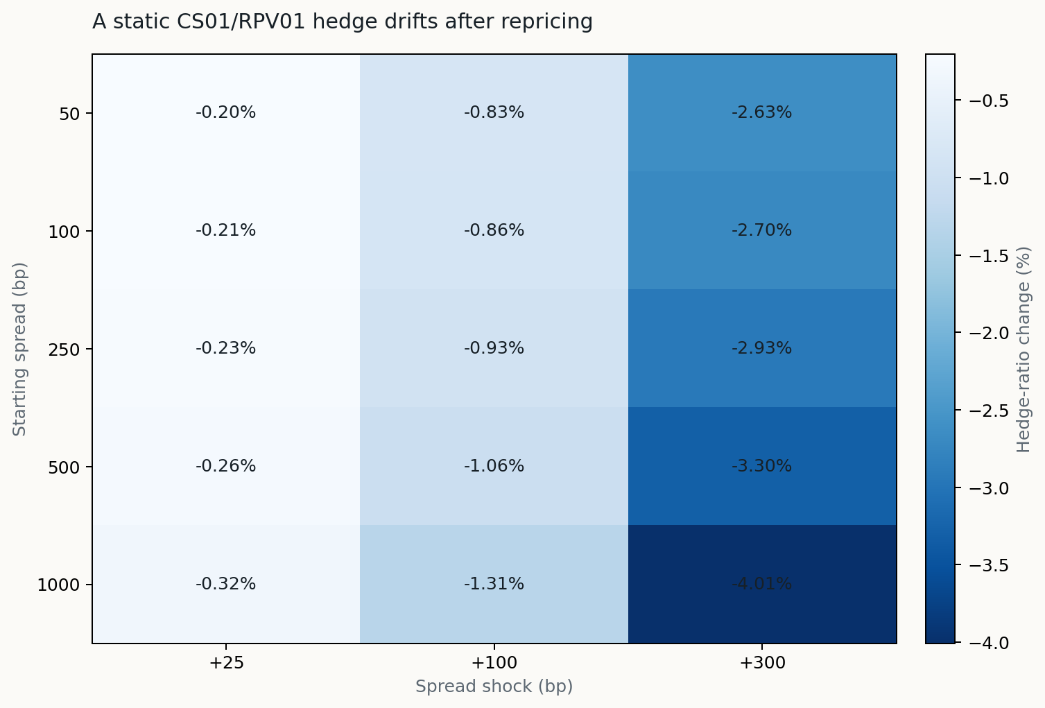
The maximum drift here is -4.01%. That does not automatically justify daily rebalancing: trading costs, liquidity and jump risk determine the rebalance policy. It does show why a backtest should recompute sensitivities and record turnover instead of treating inception hedge notionals as permanent neutrality.
What the current public data can and cannot do
The wider research repository contains actual daily equity, ETF and FRED data, plus 16 current five-year ICE Clear Credit settlement rows. Those CDS rows can exercise a standard-coupon upfront converter and produce a dated cross-sectional diagnostic.
They cannot identify a historical hazard term structure. One five-year point does not reveal the one-, three-, seven- and ten-year intervals, and one current cross-section cannot be projected backwards into a strategy history.
The honest next data steps are therefore parallel:
- collect and preserve future public settlement snapshots prospectively;
- add full-tenor licensed curves when available;
- obtain contract-level bond history and reference data;
- validate each normalized quote through the pricing engine before research;
- keep synthetic scenarios for regression tests, never as performance evidence.
From pricing engine to systematic credit research
Once historical curves exist, the same model produces better research inputs than raw spread alone:
- carry and roll-down on the hazard curve;
- curve-shape residuals against sector and rating peers;
- bond–CDS basis after model-consistent sensitivities;
- recovery and jump-to-default stress;
- equity-implied signals measured against future CDS or bond returns;
- portfolio CS01, rates DV01 and liquidity attribution.
Those signals can enter a point-in-time cross-sectional portfolio with sector, rating, issuer and liquidity constraints. Walk-forward selection, an untouched holdout, costs, turnover, deflated Sharpe and probability-of-backtest- overfitting diagnostics then become meaningful. Applying those controls to a three-event proxy test would create statistical decoration, not evidence.
The practical checklist
Before publishing a credit strategy, I now want the following questions to have explicit answers:
- Can every instrument be repriced from its stored inputs?
- Are discount, hazard, recovery and contractual conventions versioned?
- Do model quotes reproduce market quotes inside a declared tolerance?
- Are RPV01, CS01 and DV01 independently finite-difference checked?
- Is P&L fully revalued after large shocks and credit events?
- Are clean price, dirty price, accrued and upfront signs unambiguous?
- Does the hedge ratio change through time, and is rebalancing charged?
- Are real observations separated from deterministic validation scenarios?
- Has an independent implementation reproduced golden cases?
- Does the article state what the model does not price?
That is the main lesson of the exercise. A pricing engine is not merely another portfolio project. It is the part of the research process that prevents a plausible signal from borrowing credibility from an untested number.
The complete implementation, tests, deterministic experiment and guide
notebook live in research/credit-pricing-guide/. The machine-readable results
are published alongside this article so the charts and the reported numbers
come from the same run.