Research Note
Queueing Theory for Quants: Workload, Bursts and Waiting-Time Risk
Preview prompt
Summarize the Ionitsa research note titled "Queueing Theory for Quants: Workload, Bursts and Waiting-Time Risk" for a technical reader.
Cover the problem or research question, implementation or method, evidence or results, and limitations.
Separate facts stated on the page from your own assessment, note anything unclear or unverified, and avoid promotional language.

Primary source: https://ionitsa.com/research/renewal-queues-workload.md
Canonical page: https://ionitsa.com/research/renewal-queues-workload/
An interactive guide to single-server queues, workload processes and renewal arrivals, with a quant-focused explanation of capacity, burstiness, tail latency and model validation.

Queueing theory is the mathematics of what happens when random demand meets finite capacity. The visible output may be a line of customers, an order waiting for execution, a risk job waiting for compute or a payment waiting for liquidity. The underlying problem is the same: work arrives unevenly, capacity removes it, and any temporary imbalance becomes delay.
For a quant, the interesting object is not simply the average number of arrivals. It is the distribution of unfinished work and waiting time. Two systems can process the same average volume and have completely different tail latency because one receives smooth flow and the other receives bursts.
This note builds that intuition from the smallest useful model: one server, deterministic unit service and renewal arrivals. It explains the mechanics, derives the simulation, checks the Poisson case against a closed-form benchmark and shows what changes when the arrival clock is more or less variable.
Scope. This is a model laboratory, not a literal model of an exchange or a production trading stack. The assumptions are one first-come-first-served server, independent interarrival times, deterministic unit service, no cancellations and an infinite waiting room.
Why a quant should care
Queues appear throughout financial markets:
- at a price level in a limit order book, where new limit orders add depth and market orders or cancellations remove it;
- inside an execution stack, where orders pass through strategy logic, risk checks, throttles, gateways and venues;
- in market-data and research systems, where bursts of messages or jobs compete for bounded compute;
- after the trade, where allocations, confirmations, payments, collateral and exceptions compete for operational capacity or liquidity.
The analogy is not cosmetic. Limit-order-book models explicitly represent the best bid and ask as interacting queues and use order arrival, cancellation and execution intensities to study the next price move. Cont and de Larrard (2013) are a useful bridge between classical queueing and market microstructure. Payment systems also use queueing and netting mechanisms when available liquidity is scarce. BIS Project Titus is a recent institutional example.
The practical lesson is broader:
Average capacity can look comfortable while tail delay is already dangerous.
A desk that monitors only average messages per second, average tickets per analyst or average collateral movements per hour is missing the stochastic part of the risk. Capacity tells us whether the system can survive on average. The arrival distribution tells us how painful the path can be.
The right state variable is workload
A queue can be described by the number of jobs present, but workload is often the cleaner state. Let be the amount of unfinished service at time . If every job requires exactly units of service and the server processes one unit of work per unit of time, then:
- an arrival makes jump upward by ;
- between arrivals, falls with slope while it is positive;
- when the system is empty, remains at zero.
The result is a saw-tooth path. In reflected-process notation,
where counts arrivals and the non-decreasing regulator prevents workload from becoming negative.
This change of state is a quant move: choose the variable that preserves the economics while simplifying the dynamics. A count treats every item as equal. Workload measures the time or capacity required to clear what is actually there. In trading terms, ten small messages and ten expensive risk calculations have the same count but very different operational exposure.
With deterministic unit jobs, the distinction is especially transparent. Waiting time equals the workload seen on arrival, and the number of customers in the system is away from event boundaries.
Lindley’s recursion: the simulation engine
The continuous path is intuitive, but the easiest exact simulation observes the system only at arrival times. Let:
- be the gap between arrivals and ;
- be the waiting time seen by customer ;
- be the deterministic service requirement.
Then
This is Lindley’s recursion. The logic is mechanical:
- take the backlog seen by the previous customer;
- add that customer’s service requirement;
- subtract the work completed before the next arrival;
- reflect at zero because an idle server cannot create negative backlog.
In pseudocode:
wait = 0 for each interarrival gap: wait = max(0, wait + service_time - gap) record(wait)
That small recurrence is the pathwise ground truth for a GI/G/1 queue. It is fast enough to generate millions of observations and simple enough to use as a test oracle for a more elaborate density solver. The construction goes back to Lindley (1952).
Utilisation is a nonlinear risk factor
Let be the mean arrival rate. Traffic intensity is
For an infinite-buffer single-server queue, the usual stability condition is . Below one, the server has spare capacity on average. At or above one, backlog has no stationary distribution except in special degenerate cases.
The subtle point is that “below one” does not mean “safe”. For Poisson arrivals and deterministic service, the Pollaczek-Khinchine formula gives
With , the convexity is easy to see:
| Utilisation | Mean queue wait |
|---|---|
| 0.50 | 0.50 |
| 0.75 | 1.50 |
| 0.90 | 4.50 |
| 0.95 | 9.50 |
The last five percentage points of capacity are not equivalent to the first five. As approaches one, a small forecasting error or temporary burst can create a disproportionately large delay. This is the queueing analogue of convex risk: the exposure is manageable until the system moves close to a boundary, then sensitivity rises sharply.
Burstiness is a separate source of risk
Mean arrival rate is only the first moment of the flow. The experiment compares four interarrival clocks with the same :
| Clock | Interarrival construction | Squared coefficient of variation |
|---|---|---|
| Deterministic | ||
| Erlang-2 | two exponential phases, each with rate | |
| Poisson | exponential with rate | |
| Bursty lognormal | lognormal with , rescaled to mean | about |
At and unit service, perfectly regular arrivals never wait: every job reaches a server that has already cleared the previous job. Poisson arrivals have the same average volume but a theoretical mean queue wait of 1.5 time units. A high-variance clock creates longer clusters and a heavier tail.
That comparison is the central quant insight. Utilisation and burstiness are different risk factors. A capacity forecast based on average flow can be correct and the latency forecast can still be badly wrong.
The squared coefficient of variation,
is a useful first diagnostic. It is dimensionless, so flows with different time scales can be compared. It does not describe serial dependence or extreme-tail shape, but it immediately distinguishes scheduled flow from memoryless flow and bursty flow.
Two views of the same system
Pathwise view
Lindley’s recursion follows individual arrivals. It is the natural choice for Monte Carlo, stress scenarios and empirical waiting-time quantiles. It makes few numerical assumptions and exposes every sample path.
Distributional view
Sometimes we want the probability distribution over all possible workload states rather than a collection of paths. With exponential interarrivals, arrivals form a Poisson process and workload alone is Markov. For positive workload, its density can be represented schematically as
with separate treatment of probability mass at the empty boundary.
The derivative transports probability towards zero as the server works. The jump term removes probability from the current workload and adds it one service requirement higher when an arrival occurs. Numerically, this becomes a combination of a downward shift and a sparse upward-jump operator.
The two views should agree. A density method that cannot reproduce pathwise Monte Carlo and the M/D/1 benchmark has failed, however elegant its derivation looks.
What changes with non-Poisson arrivals
Exponential waiting times are memoryless. If an event has not occurred yet, the remaining time has the same distribution as it had at the start. A general renewal clock does not have that property. The probability of the next arrival depends on the age of the current interarrival interval.
Workload by itself is therefore no longer a Markov state. There are two standard ways forward:
- Augment the state. Track workload and the age of the arrival clock. The pair is Markov and can be evolved using an age-structured transport equation.
- Retain history. Eliminate the age variable and express the arrival effect as a convolution against a memory kernel.
If is the interarrival density and its Laplace transform, the renewal kernel satisfies
Hoffmann, Porter and Lambiotte (2012) developed this generalized master-equation construction for non-Poisson walks. Lai and de Kamps (2017) combined a memory kernel with characteristic-aligned bins that separate deterministic motion from random jumps.
“General” still has boundaries. A renewal process assumes independent interarrival times from one clock. Intraday seasonality, clustered order flow, self-excitation and state-dependent cancellation require richer models.
How the interactive experiment is built
The browser experiment uses the pathwise formulation, not an opaque numerical solver.
- Normalise service. Every job requires one time unit, so .
- Choose load. The traffic-intensity control sets . Because , this is also the mean arrival rate .
- Generate arrivals. Each clock samples interarrival gaps with mean , holding average demand constant.
- Draw a workload path. Over 48 time units, workload falls at unit speed and jumps by one at each arrival.
- Estimate waiting-time risk. Lindley’s recursion runs for a 1,000-arrival warm-up and retains the next 7,000 waits.
- Validate. When Poisson arrivals are selected, the empirical mean is compared with the M/D/1 formula.
The upper chart shows one realised path. The lower chart compares empirical cumulative waiting-time distributions for all four clocks at the chosen load.
Interactive experiment
One server, four arrival clocks
Hold mean load constant and change only the regularity of arrivals. The upper chart is one realised workload path; the lower chart compares empirical waiting-time distributions.
How to read the output like a quant
| Output | What it measures | Quant interpretation |
|---|---|---|
| Mean wait | average latency cost | useful, but hides the tail |
| Customers delayed | probability | frequency of capacity contention |
| Peak workload | worst backlog on one path | stress indicator, not a stable estimate |
| Waiting-time CDF | full empirical distribution | source of median, p95 and p99 latency |
| Gap between clocks | effect of flow shape at fixed mean | burstiness premium |
Do not read one random path as a forecast. The path explains mechanism; the distribution supports inference. In production research, the next step would be confidence intervals, repeated seeds, longer warm-up tests and explicit estimation error.
Four lessons from a hedge-fund quant perspective
State compression is part of the edge
The best model is often not the one with the most variables. It is the one whose state retains the risk that matters. Workload compresses an entire queue into the time required to clear it. In another setting the correct state may be queue imbalance, inventory, outstanding notional or remaining risk limit.
Averages are not distributions
Average order flow, average compute use and average operational throughput are budget numbers. Trading and risk decisions are usually made in the tails. Capacity planning should therefore pair with variance, serial dependence and high quantiles of waiting time.
Model assumptions behave like positions
Assuming Poisson arrivals is not a harmless default. It is a position on the shape and dependence of order flow. Assuming deterministic service is a position on job-size risk. A quant should know which result is driven by data and which is driven by the model’s convenience.
Validation needs an independent route
Monte Carlo, a density equation and a closed-form benchmark fail in different ways. Agreement between them is much stronger evidence than making one method more complicated. This is the same discipline used when independently rebuilding a pricing result or checking a production risk number.
From the toy queue to a market model
This G/D/1 laboratory is deliberately narrow. Extending it changes the economic question:
- random service requirements give a GI/G/1 queue and replace in Lindley’s recursion with a sampled service time ;
- multiple workers or compute nodes create a many-server queue;
- priorities represent client tiers, urgency or differentiated order types;
- finite buffers introduce blocking, rejection or dropped messages;
- time-varying rates capture the open, auctions, data releases and other intraday regimes;
- self-exciting arrivals capture clustering beyond independent renewal gaps;
- an order-book model needs at least bid and ask queues, plus limit orders, market orders, cancellations and a rule for price changes.
The point of the simple model is not realism by omission. It is identification: first isolate utilisation and interarrival variability, then add market mechanisms one at a time.
Personal reference and source artifact
This page grew from a student project and the QueueingTheory repository. The original poster is preserved below as a personal reference and a record of the initial route from population-density methods to queueing. Its historical title, A novel algorithm for G/D/1 queues, should not be read as a current novelty or validation claim.
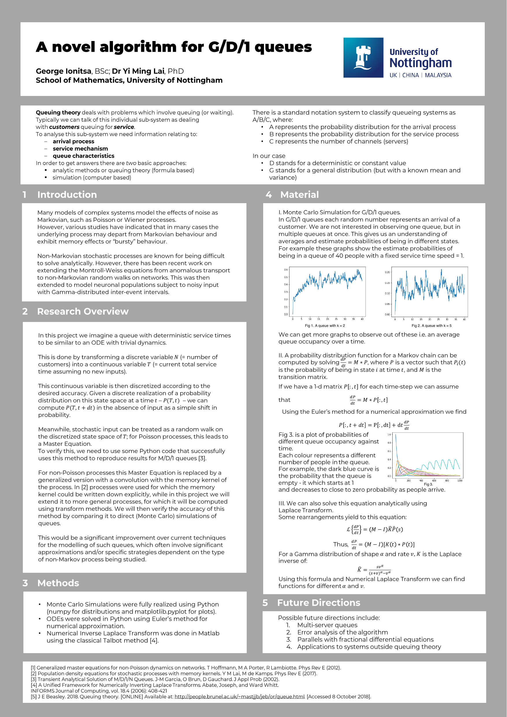
Open the original poster as a PDF
The current page does not reuse the poster’s unfinished renewal solver. It rebuilds the pathwise queue from Lindley’s recursion, makes every distributional assumption visible and benchmarks the Poisson case against established theory. That is the distinction between preserving an idea and relying on an old numerical result.
AI-assisted research reconstruction
Modern coding models make this kind of personal research archaeology much less expensive. They can trace legacy code, recover assumptions, translate obsolete syntax, generate tests and help compare an implementation with known results. A 2025 Wiley survey reported that 84% of surveyed researchers had used AI tools in their work and 62% had used them for research or publication tasks. Wiley, ExplanAItions 2025
AI was used here as a research and implementation assistant, not as an authority that could declare the mathematics correct. The standard remains reproducible code, explicit assumptions and independent checks. The useful workflow is not “ask a model whether this is right”; it is “use a model to make the work cheap enough to rerun, inspect and try to falsify.”
Conclusion
Queueing theory gives quants a compact language for capacity risk. Workload is the state, measures average pressure, the arrival distribution controls burstiness, and the waiting-time distribution records the cost.
The deepest lesson is that equal average flow does not imply equal risk. A smooth stream, a Poisson stream and a clustered stream can consume the same capacity while producing radically different delay profiles. That principle travels well—from order books and execution systems to compute, operations, payments and collateral.
Sources
- D. V. Lindley, “The Theory of Queues with a Single Server”, Mathematical Proceedings of the Cambridge Philosophical Society 48(2), 1952.
- R. Cont and A. de Larrard, “Price Dynamics in a Markovian Limit Order Market”, SIAM Journal on Financial Mathematics 4(1), 2013.
- T. Hoffmann, M. A. Porter and R. Lambiotte, “Generalized Master Equations for Non-Poisson Dynamics on Networks”, Physical Review E 86, 046102, 2012.
- Y. M. Lai and M. de Kamps, “Population Density Equations for Stochastic Processes with Memory Kernels”, Physical Review E 95, 062125, 2017.
- Bank for International Settlements, “Project Titus: Market-Based Liquidity Efficiency in RTGS Systems”, 2025.
- G. Ionitsa, QueueingTheory source repository, personal project materials.