Research Note
When Equity Moves First: A Public-Data Equity–Credit Stress Test
Preview prompt
Summarize the Ionitsa research note titled "When Equity Moves First: A Public-Data Equity–Credit Stress Test" for a technical reader.
Cover the problem or research question, implementation or method, evidence or results, and limitations.
Separate facts stated on the page from your own assessment, note anything unclear or unverified, and avoid promotional language.

Primary source: https://ionitsa.com/research/when-equity-moves-first.md
Canonical page: https://ionitsa.com/research/when-equity-moves-first/
A three-year, 16-issuer study of whether broad idiosyncratic equity shocks precede credit stress, with next-close execution, randomization tests, block-bootstrap Monte Carlo and an honest account of the data still required for issuer CDS and bond trading.
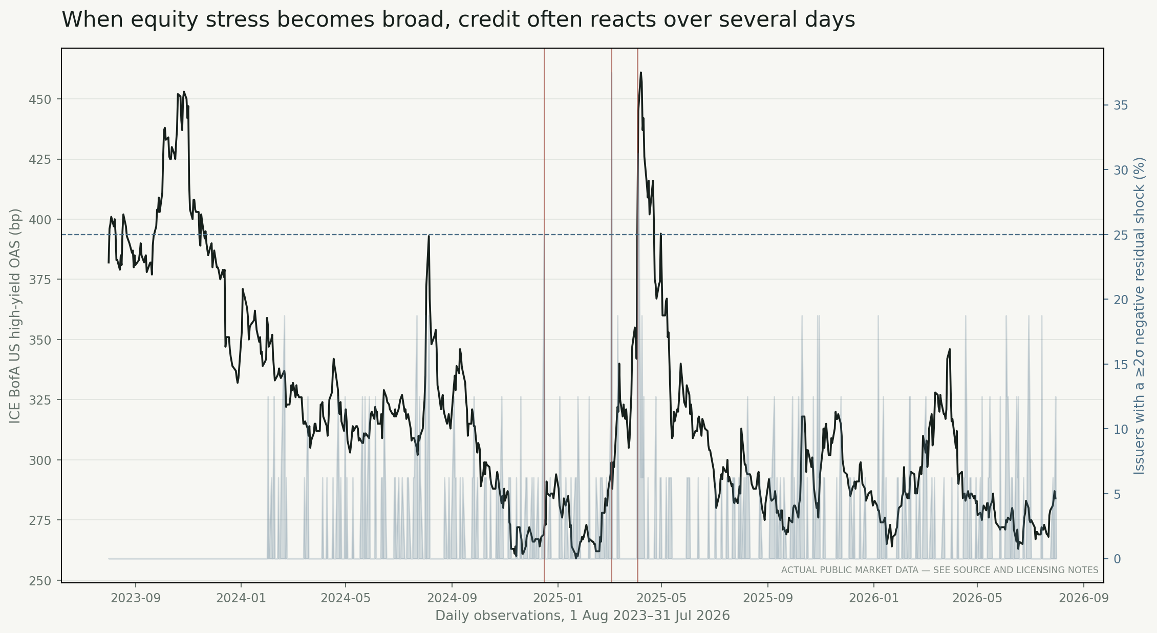
When a company’s equity price falls sharply, its creditors have learned something too. The difficult question is whether the equity market learned it first.
That distinction is the basis of a capital-structure strategy. Equity trades continuously on a centralized venue. Corporate bonds are split across issues and trade over the counter. A credit default swap isolates credit risk but is a separate legal contract with its own liquidity, documentation and pricing conventions. Information can reach those markets at different speeds.
This study asks a deliberately narrower first question: when idiosyncratic equity stress becomes broad across companies, does the liquid credit market tend to deteriorate over the next several days?
The pilot uses actual daily public observations for 16 US and European issuers, four traded market proxies and four macro-credit series from 1 August 2023 to 31 July 2026. It combines an event study, a timing-safe HYG hedge test, a random event benchmark, block-bootstrap Monte Carlo and a separate comparison with current ICE single-name CDS settlements.
The headline result is promising but intentionally qualified. Only three non-overlapping events passed the baseline stress rule. Five days later, high-yield OAS had widened in all three cases by an average 26.7 basis points, and HYG had lost an average 1.38%. A HYG short executed at the next close and measured only after that execution returned 1.55% net of a five-basis-point round-trip assumption. That is enough to justify a larger licensed-data study. It is nowhere near enough to claim a finished strategy.
What is actual data—and what is not
The historical dataset contains 12,048 daily issuer observations, or 753 trading days for each of 16 equity lines. US issuers use their US common shares. European issuers use active US-listed ADRs or US trading lines so that all returns share a consistent trading calendar.
| Region | Issuers and equity symbols |
|---|---|
| US | Ford (F), Boeing (BA), AT&T (T), Verizon (VZ), IBM (IBM), Carnival (CCL), Delta Air Lines (DAL), AIG (AIG) |
| Europe | ArcelorMittal (MT), Sanofi (SNY), Philips (PHG), Ericsson (ERIC), Nokia (NOK), Stellantis (STLA), TotalEnergies (TTE), Eni (E) |
Daily prices came from Nasdaq’s public historical-price service. SPY and VGK represent broad US and European equity conditions; HYG and LQD represent liquid US high-yield and investment-grade credit. FRED contributes the ICE BofA US Corporate OAS, ICE BofA US High Yield OAS, the five-year Treasury yield and VIX.
ICE’s public five-year single-name settlement page contained 1,114 contracts at retrieval. The study exact-matched 16 senior 100-basis-point-coupon contracts by reference entity, tier, currency, documentation clause and maturity.
There is a crucial boundary in the evidence:
- the equity, ETF and FRED series are actual daily histories;
- the ICE single-name CDS data is one current settlement cross-section;
- it is not a historical issuer-level CDS spread series;
- the ICE EOD field is retained as a price and is never relabelled as a par spread;
- no historical bond-price or TRACE trade panel is used in this pilot.
The original downloads and normalized observations remain local because source terms can restrict redistribution. The code publishes an immutable manifest of URLs, retrieval time, row counts and SHA-256 hashes, plus aggregate outputs and figures. This makes the work reproducible without pretending that public pages provide an institutional security master.
Nasdaq closes in this extract are unadjusted price observations. They therefore omit dividends and can differ from total returns. The European lines are ADRs, not primary European closes. Both choices are acceptable for a pilot shock signal, but neither should survive unchanged into a production strategy.
From an equity move to an issuer shock
A raw equity decline is not enough. If the whole market falls 3%, a 3% issuer loss contains little company-specific information. Each issuer is therefore measured against its regional market proxy.
For issuer on day , the residual return is
where is the SPY return for US names or the VGK return for European names. The beta estimate uses the preceding 63 observations and is shifted by one day. Today’s return never enters today’s beta.
The issuer-level shock indicator is
where is prior 63-day residual volatility. Daily shock breadth is the fraction of eligible issuers in shock:
The baseline rule is intentionally simple:
| Parameter | Baseline value |
|---|---|
| Market-beta lookback | 63 trading days |
| Negative residual shock | at least 2 prior standard deviations |
| Breadth trigger | 25% of issuers |
| Event cooldown | 10 trading days |
| Hedge | short HYG |
| Holding period | 5 trading days |
| Execution | next close; first P&L after that close |
| Round-trip cost | 5 basis points |
This is a market-stress hedge test, not yet a single-name arbitrage. HYG is used because it supplies a real, timestamped and executable public history. Replacing it with issuer CDS or a selected corporate bond requires historical quotes, contract sensitivities and transaction-cost data that the public CDS snapshot does not contain.
What happened after the three signals
The 25% breadth threshold generated three non-overlapping events: 16 December 2024, 4 March 2025 and 3 April 2025.
| Forward horizon | Mean HY OAS change | Events with wider OAS | Mean HYG return | Events with HYG loss |
|---|---|---|---|---|
| 1 trading day | +13.0 bp | 2 of 3 | -0.53% | 2 of 3 |
| 5 trading days | +26.7 bp | 3 of 3 | -1.38% | 3 of 3 |
| 10 trading days | +16.0 bp | 3 of 3 | -0.70% | 3 of 3 |
The path matters. On 4 March 2025, high-yield OAS tightened 11 basis points on the first day, then widened 23 basis points by day five. On 3 April, it widened 44 basis points immediately and 41 basis points over five days, but nearly all of that widening had reversed by day ten. The signal does not describe a permanent repricing. It describes a possible multi-day window in which credit stress catches up and then may mean-revert.
The baseline hedge earned 1.55% net over 15 invested days. Mean trade return was 0.52%, median trade return 0.78%, two of three trades were positive and maximum drawdown was -2.68%.
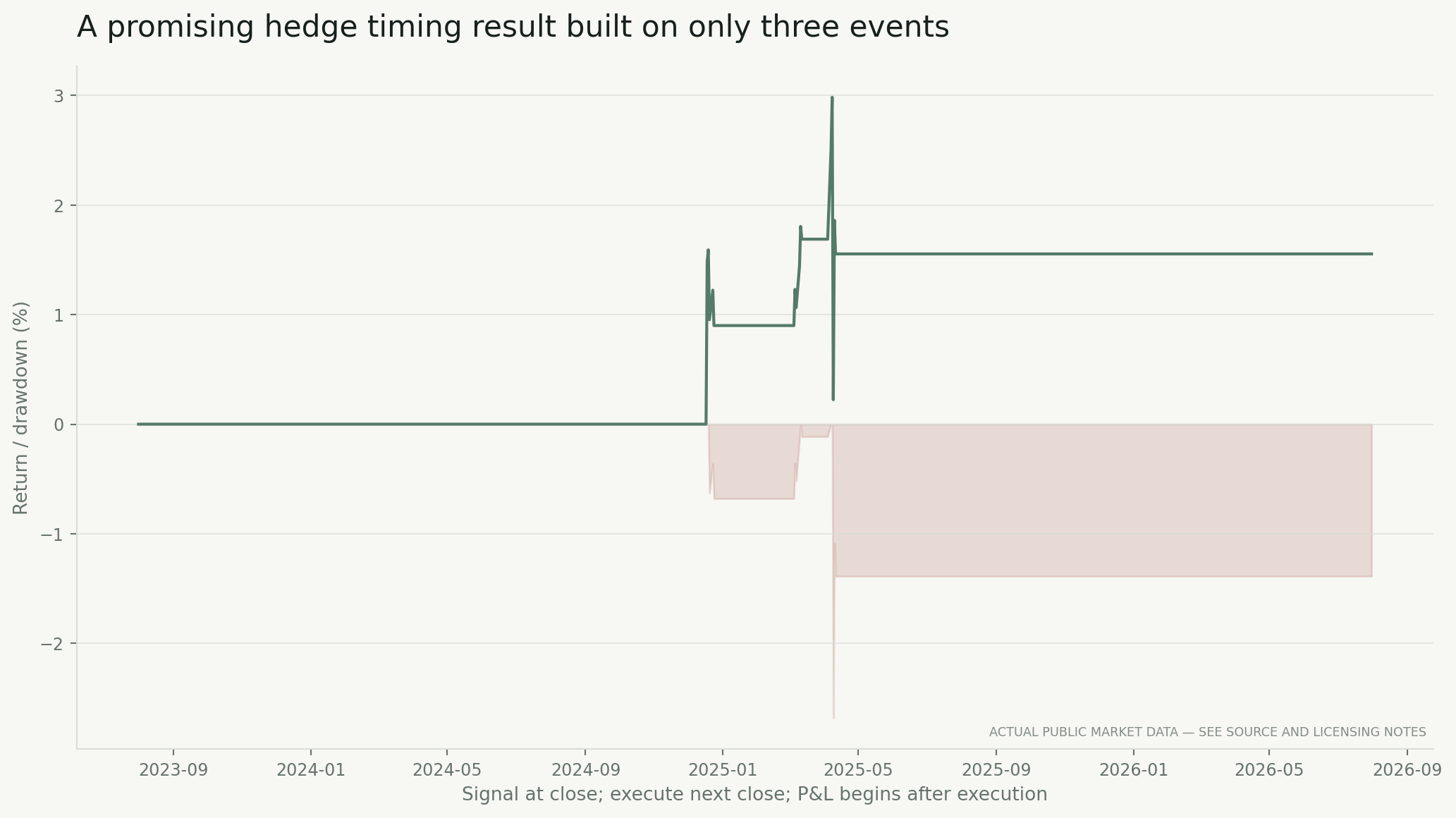
Those numbers should not be annualized into a marketing Sharpe ratio. The strategy is inactive on almost every day, the event count is three, and all signals come from a short modern sample. A single losing event could materially change every statistic.
Does the result survive nearby specifications?
A useful signal should not exist at only one magical parameter combination. I therefore varied breadth thresholds from 12.5% to 31.25% and holding periods from one to ten days while retaining next-close execution and the same cost assumption.
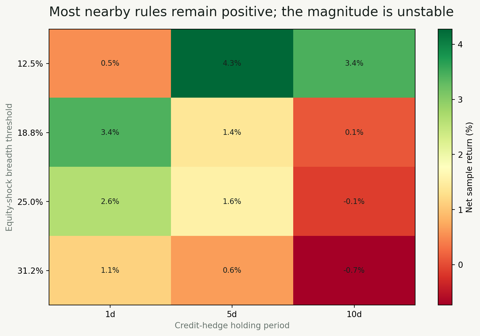
The five-day rule was positive at every threshold: 4.27%, 1.40%, 1.55% and 0.65% across the four breadth cutoffs. One-day returns were also positive. The ten-day rule turned slightly negative at the two highest thresholds.
That pattern is economically coherent with a delayed credit response, but the magnitude is unstable. The lowest threshold produces 31 events and a much smaller average trade. The highest produces only two. This is a robustness surface, not a search for the best cell; selecting the 4.27% result after seeing the table would be data mining.
Monte Carlo: three simulations, three questions
“Monte Carlo” is not one method and it does not manufacture evidence. It is a way to ask how a statistic behaves under an explicit resampling model.
1. Random event timing
The first test draws 10,000 sets of three random, non-overlapping event dates, applies the same next-close five-day HYG short and subtracts the same cost. The actual mean trade return was 0.52%. Random timing produced a median of -0.10% and a 95% interval from -0.88% to +0.72%. About 6.08% of simulated samples matched or exceeded the actual mean, giving a one-sided randomization p-value of 0.0608.
This answers a narrow question: the selected dates were unusually favorable for short-HYG positions relative to arbitrary dates in the same history. It does not prove that the signal will work in a new regime, because the dates were still generated by one three-year market path.
2. Moving-block strategy bootstrap
The second test resamples ten-day blocks of the realized strategy return series 10,000 times. Blocks preserve short clusters of volatility and dependence that an independent daily bootstrap would destroy. The median simulated total return was 1.47%, with a 95% interval from -1.52% to 5.14%; 82.3% of paths finished positive. The median simulated maximum drawdown remained -2.68%.
This result looks supportive, but most observations are zero because the hedge is rarely active. The simulation repeatedly reuses the same three episodes. It measures uncertainty inside the observed path; it cannot invent a credit crisis, a CDS liquidity break or a different inflation and rates regime.
3. Cross-sectional equity tail bootstrap
The third test samples common five-day blocks across all 16 equities and joins four blocks into 20-day paths. Sampling the same dates across names preserves their contemporaneous dependence. For each issuer, 10,000 paths estimate the probability of losing at least 10%, the fifth-percentile return and expected shortfall beyond it.
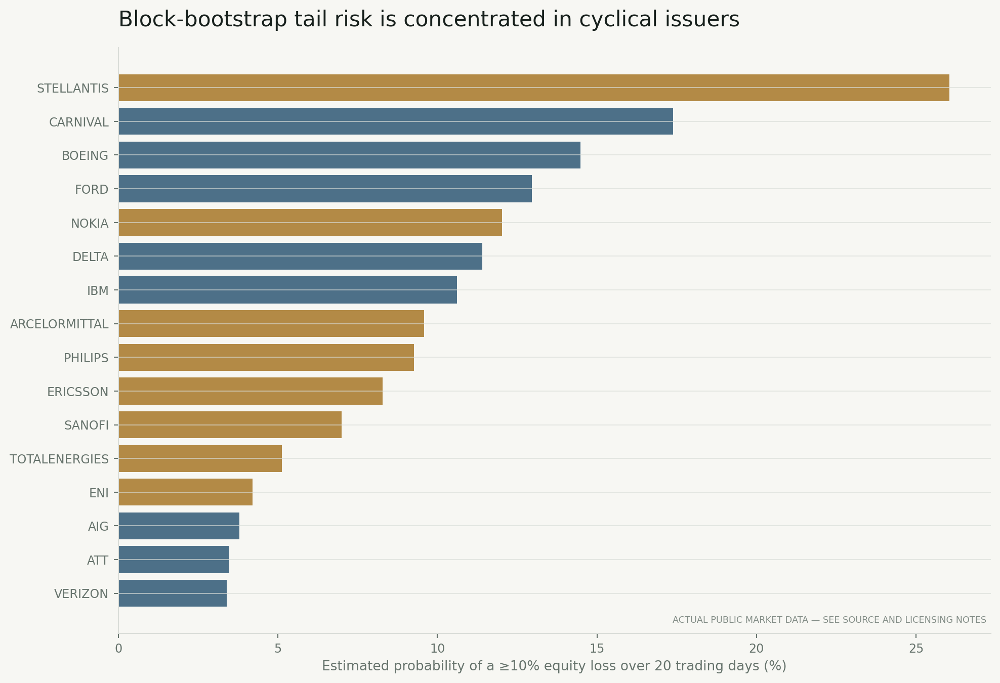
Stellantis had the largest estimated probability of a 10% loss at 26.0%, with a fifth-percentile outcome of -22.1% and expected shortfall of -27.7%. Carnival followed at 17.4%, Boeing at 14.5% and Ford at 13.0%. Verizon and AT&T were near 3.4%–3.5%.
These are historical conditional distributions, not probabilities of default and not forecasts from a structural credit model. Their value is relative: they identify issuers for which an equity-triggered credit hedge is most likely to encounter convex, nonlinear outcomes.
Does current CDS pricing agree with equity distress?
The ICE snapshot provides a separate cross-sectional check. I combine trailing 63-day realized and downside volatility, 63-day momentum and current 252-day drawdown into a within-region equity distress score. I then compare that score with the discount of the standardized ICE CDS settlement price to par.
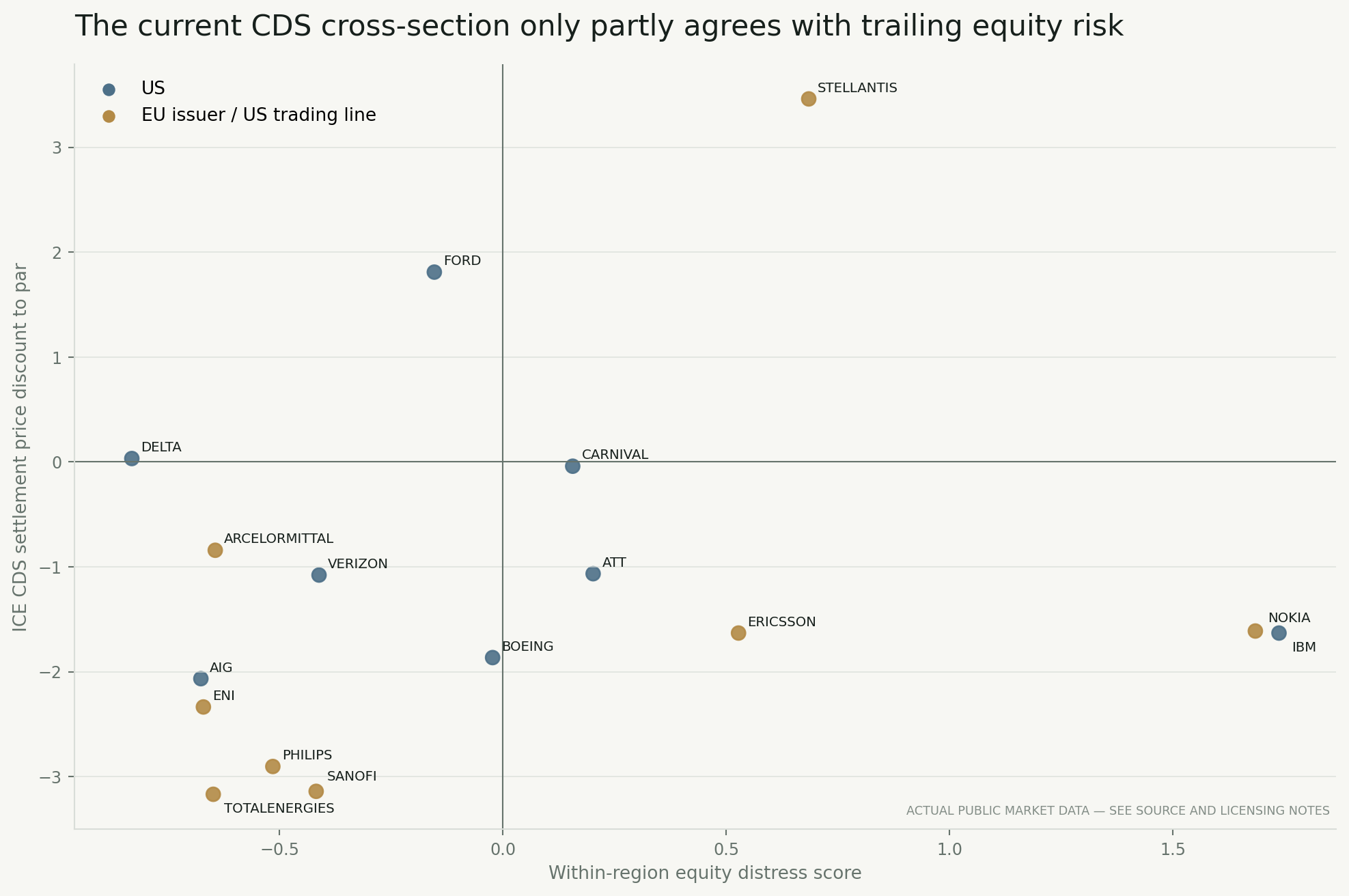
Across all 16 issuers, the Spearman rank correlation was 0.30. The EU subset was 0.50; the US subset was -0.10. A 10,000-draw pairs bootstrap put the pooled median at 0.29, but its 95% interval ran from -0.26 to 0.70. The interval crosses zero because 16 observations cannot identify a stable relationship.
This mixed result is important. The strong aggregate stress timing does not automatically imply strong issuer selection. Broad equity shocks may say something useful about the next move in the credit factor while a simple cross-sectional equity distress score says little about which standardized CDS contract is rich or cheap today.
Why bonds and CDS are the harder second stage
A real three-asset test needs more than prices. For every date and issuer it needs a legally and economically consistent mapping among the equity issuer, bond obligor, CDS reference entity and ultimate parent. A parent equity can be paired with subsidiary debt, but that is a model choice—not a name match.
The bond leg needs clean and dirty price, accrued interest, OAS or par-equivalent spread, CS01, DV01, trade volume, bid/ask, amount outstanding, quote freshness and borrow. FINRA publishes TRACE reference and transaction data under its fixed-income data framework, but trade prints are not executable quotes and historical availability and terms require careful handling. European instruments can be discovered through ESMA’s FIRDS reference files, but issuer hierarchy and liquidity still have to be built.
The CDS leg needs par spread or upfront, recovery convention, RPV01, bid/ask, tier, currency, restructuring clause, contract maturity, roll treatment and a point-in-time reference-entity mapping. DTCC’s public OTC repository reports are useful evidence of single-name activity; they are not a clean daily tradable spread curve.
Once those inputs exist, the strategy can graduate from a broad credit hedge to three issuer-level tests:
- Equity-to-CDS delay: buy protection when negative equity residuals have not yet appeared in CDS, and test the reverse direction as a falsification.
- Equity-to-bond delay: short or underweight a liquid bond when equity deterioration has not reached OAS, controlling duration and curve exposure.
- Equity-gated bond–CDS basis: use equity distress and recovery states to time a matched bond-plus-CDS relative-value trade.
The hedge ratios cannot be dollar matched. Equity beta to firm value, bond CS01 and DV01, and CDS RPV01 must be estimated separately. Jump-to-default, recovery, volatility skew, curve risk, financing and cheapest-to-deliver optionality remain even after first-order hedging.
What would falsify the strategy
The next study should reject the hypothesis if the effect disappears when:
- daily issuer CDS and bond quotes replace broad HYG and OAS proxies;
- the universe is reconstructed point in time with defaults, delistings, mergers and CDS succession events preserved;
- stale credit marks and earnings-day discontinuities are isolated;
- signal formation and execution timestamps are enforced at intraday precision;
- bid/ask, financing, bond borrow, CDS roll and failed-trade costs are charged;
- crisis and calm regimes are tested separately;
- or the rule is evaluated on issuers and dates never used in its design.
The three-event pilot has done its job: it found a coherent relationship worth testing and exposed exactly where the public-data boundary lies. The next level is not a more elaborate simulation of the same sample. It is a longer, point-in-time, issuer-level CDS and bond panel with executable transaction-cost assumptions and a genuinely untouched out-of-sample period.
The retrieval, analysis and test code is maintained in the companion Equity–Credit Capital Structure Strategies project. All figures and numerical results above are generated from the dated replication pipeline. This is research, not investment advice.